Plot trial metric history

Plots the history of relevant metrics over the progress of a single or multiple trial simulations. Simulated trials only contribute until the time they are stopped, i.e., if some trials are stopped earlier than others, they will not contribute to the summary statistics at later adaptive looks. Data from individual arms in a trial contribute until the complete trial is stopped.
These history plots require non-sparse results (sparse set to FALSE; see run_trial() and run_trials()) and the ggplot2 package installed.

Usage

plot_history(object, x_value = "look", y_value = "prob", line = NULL, ...)

# S3 method for trial_result
plot_history(object, x_value = "look", y_value = "prob", line = NULL, ...)

# S3 method for trial_results
plot_history(
  object,
  x_value = "look",
  y_value = "prob",
  line = NULL,
  ribbon = list(width = 0.5, alpha = 0.2),
  cores = NULL,
  ...
)

Arguments

object

trial_results object, output from the run_trials() function.

x_value

single character string, determining whether the number of adaptive analysis looks ("look", default), the total cumulated number of patients randomised ("total n") or the total cumulated number of patients with outcome data available at each adaptive analysis ("followed n") are plotted on the x-axis.

y_value

single character string, determining which values are plotted on the y-axis. The following options are available: allocation probabilities ("prob", default), the total number of patients with outcome data available ("n") or randomised ("n all") to each arm, the percentage of patients with outcome data available ("pct") or randomised ("pct all") to each arm out of the current total, the sum of all available ("sum ys") outcome data or all outcome data for randomised patients including outcome data not available at the time of the current adaptive analysis ("sum ys all"), the ratio of outcomes as defined for "sum ys"/"sum ys all" divided by the corresponding number of patients in each arm.

line

list styling the lines as per ggplot2 conventions (e.g., linetype, linewidth).

...

additional arguments, not used.

ribbon

list, as line but only appropriate for trial_results objects (i.e., when multiple simulations are run). Also allows to specify the width of the interval: must be between 0 and 1, with 0.5 (default) showing the inter-quartile ranges.

cores

NULL or single integer. If NULL, a default value set by setup_cluster() will be used to control whether extractions of simulation results are done in parallel on a default cluster or sequentially in the main process; if a value has not been specified by setup_cluster(), cores will then be set to the value stored in the global "mc.cores" option (if previously set by options(mc.cores = <number of cores>), and 1 if that option has not been specified.
If cores = 1, computations will be run sequentially in the primary process, and if cores > 1, a new parallel cluster will be setup using the parallel library and removed once the function completes. See setup_cluster() for details.

Value

A ggplot2 plot object.

See also

plot_status().

Examples

#### Only run examples if ggplot2 is installed ####
if (requireNamespace("ggplot2", quietly = TRUE)){

  # Setup a trial specification
  binom_trial <- setup_trial_binom(arms = c("A", "B", "C", "D"),
                                   control = "A",
                                   true_ys = c(0.20, 0.18, 0.22, 0.24),
                                   data_looks = 1:20 * 100)



  # Run a single simulation with a fixed random seed
  res <- run_trial(binom_trial, seed = 12345)

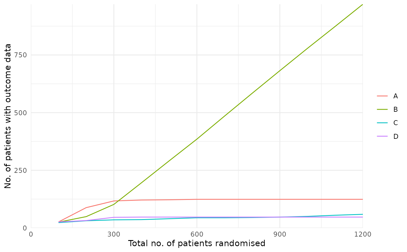
  # Plot total allocations to each arm according to overall total allocations
  plot_history(res, x_value = "total n", y_value = "n")

}


if (requireNamespace("ggplot2", quietly = TRUE)){

  # Run multiple simulation with a fixed random base seed
  # Notice that sparse = FALSE is required
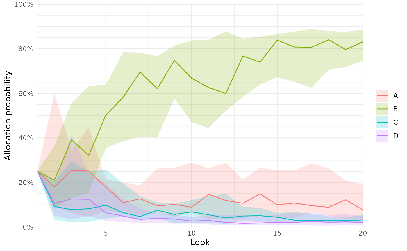
  res_mult <- run_trials(binom_trial, n_rep = 15, base_seed = 12345, sparse = FALSE)

  # Plot allocation probabilities at each look
  plot_history(res_mult, x_value = "look", y_value = "prob")

  # Other y_value options are available but not shown in these examples

}